Zero-Knowledge Proofs: A Technology Primer
- 1. Introduction
- 2. Why do we care?
- 3. Zero-knowledge Proofs
- 4. History of ZKPs
- 5. Applications of ZKPs
- 6. Appendix
Introduction
In recent months, zero-knowledge proofs have seen both significant academic development and impactful practical implementations across crypto. From zero-knowledge rollups to private chains, major advances are being made towards developing novel products and increasing usability for existing ones. The speed of development in this area can quickly obscure the progress that has been made. The purpose of this report is to set out the current state of research, discuss the most recent developments, and explore the practical implementations of said research.
Why do we care?
Zero-knowledge proofs are primarily used for two things: Ensuring computations are correct, and enforcing privacy.
- 1. Verifiable computation is a method of proving that we have correctly performed a calculation. We can use such technology to design scalability solutions, such as zero-knowledge rollups, as well as other novel structures like shared execution layers. The zero-knowledge rollup sector has seen a significant leap in traction driven by their provision of a solution to the particularly high fees and low throughput on certain L1s such as Ethereum. Verifiable computation has its applications off-chain as well – for example, proving that a critical program (e.g. one that outputs medical decisions or directs large financial transactions) has executed correctly, so that we are
sure no errors have occurred. The key here is that we can verify in milliseconds the execution of a program that might have originally taken hours to run, rather than having to check it by re-running. - 2. Privacy is another major feature, and one that may prove vital in inducing widespread adoption. Zero-knowledge proofs can be used to attest to the validity of private transactions, allowing us to maintain trustlessness and consensus without disclosing the contents of any transaction. Naturally, this does not only have to happen on the base layer – this could be implemented in an off-chain context, generating/verifying the proofs on individual devices, which might be more suitable in cases where we care more about costs and less about decentralization.
In this report, we focus on the first of these, exploring the state of research surrounding zero-knowledge proofs, their implications, and the potential focus of future works.
Zero-knowledge Proofs
Zero-knowledge proofs (“ZKPs”) are a cryptographic method of proving whether or not a statement is true without giving away any other information.
For example, consider the following, in which we want to show someone that we know where Wally is, yet do not want to reveal the location itself [1].


What we might do is take a very large sheet of paper, cut a small hole in it, and position the hole over Wally. Then anyone we show can see that we have indeed found Wally, yet they don’t gain any information about where he is, as they cannot see the rest of the page, and the page could be anywhere under the sheet.
Alternatively, suppose that there is a circular cave with a locked door, and Alice wants to prove to Bob that she has the password without giving it (or any other information) up [2].
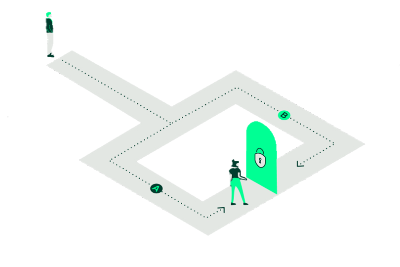
Alice enters the cave and goes down one of the two paths, A or B. Then Bob, without knowing which she has picked, enters the cave and shouts out a direction, again A or B, choosing at random. If Alice does indeed know the password, then she can exit from the correct path every time, simply passing through the door if Bob called out the path opposite to the one she is in. If, however, she does not know the password, then since Bob is calling out a random path, she will only be able to exit from the same path he called with a probability of 50%. If the two repeat this process many times, Bob will be able to confirm whether or not Alice has told the truth with a high probability, all without disclosure of the password. Moreover, Bob cannot replay some recording of this to a third party and convince them of the same fact, since if the two had colluded and agreed beforehand the order in which the paths would be called out, they could fake that proof.
Notably, if Bob simply entered the cave and observed Alice coming out from a different path than she entered, this would also be a proof that she knows the password without her disclosing it. However, now Bob has learnt something new – if he records their interaction, he now knows how to prove to other people that Alice knows the password. This means that the proof is no longer zero-knowledge, because zero-knowledge proofs are designed to not reveal any information other than the truth of their statement. In this case, we need some randomness or interaction in order to prevent this from happening.
A more technical example of a ZKP is that of proving that you know the discrete logarithm of a given value. To motivate this, we might consider a scheme where Alice wants to prove to Bob that she knows a certain password without revealing to him (or anyone) what that password is. Letting be some integer, a large prime, and some positive integer less than , Alice wants to prove to Bob that she knows an integer such that . The former is her password, and the latter is information that has been shared by Alice prior so that she can verify the password later.
The two repeat these steps until Bob is satisfied:
- 1. Alice picks a random integer uniformly over and calculates , sending it to Bob.
- 2. Bob chooses randomly either or to ask Alice to send to him.
- 3. In the first case, Bob verifies . In the second, he verifies .
If Alice does not know , then she fails when Bob asks her to send the second value in step 2, so she fails 50% of the time. After n repeats, she has only a chance of fooling Bob. Eventually, he would consider this satisfactory.
If she knows in advance which will be chosen, she can falsify the proof by sending, in step 1, in the first case, and alongside r' instead of x+r in the second case, passing the verification check – so, in fact, nobody watching this process is convinced that Alice has the information she claims (since Alice and Bob may be conspiring – in practice, they might conspire to fake proofs of transactions and steal money). More than that, this means that any information that Bob gets from the process, he could have calculated himself from the public information (and some random values), since he knows what he will pick – meaning that he cannot obtain any knowledge from the process at all.
The applications of ZKPs are wide-ranging. Perhaps you want to prove that your credit score is high enough for a loan without telling the lender what your score actually is. Perhaps you want to prove that a block you’ve constructed is valid – and more than this, you want to hide the content of the transactions. Across Web2 and Web3, there are vast opportunities for applications of ZKPs where people want trustlessness, security, and privacy simultaneously.
Of course, the example we described is limited to a single statement. We can generalise this to a large extent. For example, ZKP systems can be created that provide proofs for many computational statements e.g. “I know x such that ” – an example of such a system being Succinct Non-Interactive Arguments of Knowledge (SNARKs, 3.6), which are particularly popular.
The above example of a polynomial is an instance of a wider problem – the one of finding the roots of a general polynomial. This is an NP problem, i.e. it is somehow hard to solve yet easy to verify. Many general systems are ‘universal’ in that they can be used to prove general computations (languages) in NP (and in some cases a broader range of problems).
Going forward, we refer to the party that generates the ZKP (Alice’s role) as the ‘prover’ and the party being proved to (Bob’s role) as the ‘verifier’.
3.1 Arguments of Knowledge
To give some context to the discussion of ZKPs, we talk about arguments of knowledge (“ARKs”), a generalisation of ZKPs.
An argument of knowledge is any way for a prover to convince a verifier of a fact, in which the prover can only realistically do so convincingly if the fact is true.
The obvious way of doing this is to show someone a direct proof of the fact. For example, in our ‘Where’s Wally’ proof, we could just point to Wally in the book. We refer to this as the ‘trivial proof’. However, for our purposes, this is relatively uninteresting (since it is the obvious answer with no special properties), so we mostly focus on arguments of knowledge that are somehow faster or shorter, or can be turned into a ZKP by some method.
By faster or shorter, we mean cases where the amount of communication for the proof is smaller, the time taken [3] for the prover to generate the proof is shorter, or the time taken to verify the proof is shorter – in each case comparing to the same for the trivial proof. For example, the Wally proof takes longer than simply pointing him out, but is zero-knowledge.
Of course, if the proof system is not any of these, and is not a zero-knowledge proof, this is not interesting – the trivial proof is automatically better than what we have.
The importance here is that an argument of knowledge is not necessarily a ZKP. Achieving zero-knowledge is no simple task, because any leak of information breaks it. Sometimes the condition of zero-knowledge is unnecessary for our purposes, but when it becomes important, it is vital that the distinction is drawn. For example, if we want to prove that a block of Ethereum transactions is valid, then we only care about the computational savings, not ZK (since the information is all public).
However, in the Alice/Bob example, if information about Alice’s password can be extracted from her proof, then it makes it easier for any malicious party to steal her identity, so ZK is vital.
3.2 (Non-) Interactive Proofs
We can divide the examples of ZKPs from earlier into two types:
- 1. Our ‘Where’s Wally’ proof is non-interactive, meaning that the only communication is one message from the prover to verifier consisting of a self-contained proof.
- 2. The discrete log example is interactive, meaning that the proof consists of a number of rounds of communication between the prover and the verifier.
Interactive proofs are typically easier to construct (especially for high levels of security), and serve as a foundational building block of many proof systems. However, they lack convenience. For example, if I want to prove to the world that I have a valid transaction, I don’t want to have to communicate with every person that wants to confirm this. Non-interactive proofs are exceedingly helpful as they avoid this problem entirely.
Moreover, a non-interactive proof can be verified at any time without the participation of the prover, meaning that proving and verifying can be done asynchronously.
If we write an interactive proof that uses public randomness, we can turn it into a non-interactive one (and indeed this is how some major implementations have been formed) using a process called the Fiat-Shamir heuristic. In essence, we replace the randomness with some kind of pseudo-random function, like a hash function, for which if we know the inputs we can check it was generated correctly.
An important note here is that the randomness must be public. If the randomness needed to be private, to stop the prover from falsifying a proof, then letting them use a hash function instead would allow them to pre-compute the randomness and use it maliciously. Let’s take our discrete log example. We have already established that if Bob’s random choice is known to Alice, then she can generate a false proof. If Alice uses a hash function in the place of Bob (i.e., a pseudo-random function outputting 0 or 1 to pick between the two requests), then she will be able to predict the coin toss by calculating the result in advance, at which point she could generate a false proof.
3.3 Scalability and Succinctness
As mentioned previously, we want to consider arguments of knowledge that scale nicely in two main regards.
Firstly, the proof length and the verifier time. We refer to an ARK as ‘succinct’ if the proof size and verification time are at worst polylogarithmic in the time taken to verify the trivial proof. In other words, we must be able to bound the proof size and verification time by a certain polynomial in , where is the time taken to check the trivial proof. Put another way, the proof size and verification time grow quite a bit slower than the trivial proof does. In essence, a succinct ARK is typically quite a bit faster in convincing the verifier than the trivial proof (not including the prover time).
Note that a polynomial is anything of the form , where the a’s are constant.
Now we consider the prover. An ARK is ‘scalable’ if it is both succinct and has a prover time that is quasilinear in the running time of the trivial proof. In other words, the prover time can be bounded by for some constant . This isn’t quite as good as the bound we had for succinctness, but it still stops the prover time from growing too quickly – something that can happen when trading off for verifier efficiency. It also doesn’t make a comparison with the time it took to generate the trivial proof; rather it just imposes a bound on how fast the prover time is allowed to scale.
Achieving either of these is desirable – it means that (in both cases) we can introduce manageable overhead for the prover and moreover (in the second case) factually beat the obvious method of proving a statement when considering the perspective of the verifier.
3.4 Arithmetizations & Circuits
When we want to create a ZKP for a computation, we often want to put it in a standardized form that is easier to work with (or the form that the chosen ZKP requires). The method that we choose to do this in is called an arithmetization, and the application of that method to a specific computation is called a circuit.
What we’re doing here is effectively refining the computation into a form we can use. When we get ore out of the ground, we put it through a few processes to refine it into solid metal that we can then make products with – and that’s analogous to what an arithmetization does for a computation.
The reason that we do this is to support the development of general proof systems. We don’t want to have to design a new ZKP every time we come up with a new statement, as this would require a significant amount of time and effort. Having a specific form with which to write computations allows us to more easily reason about what we can do to that end. Moreover, we can design the arithmetization to work well with our method for introducing zero-knowledge. For example, Rank 1 Constraint Systems (“R1CSs” – see below) allow us to turn a computation into a set of polynomials, which we can (relatively) easily encrypt with elliptic curves, introducing zero-knowledge.
There are two commonly used arithmetizations: R1CS and Plonkish. We will cover both here, but a deeper description of each will be included in the appendix.
R1CS was the arithmetisation used for the original SNARK implementations. It is a versatile method of expressing a computation as a set of polynomials, able to express NP problems, and so continued to be used for a while. However, with the release of PLONK [4] and related works, it became clear that R1CS had its drawbacks, such as a lack of flexibility (individual constraints were less expressive than Plonkish, making R1CS less efficient) leading to Plonkish arithmetizations becoming the preferred standard (where suitable).
3.4.1 R1CS
The R1CS (May 2013) is a form of arithmetisation commonly used for Succinct Non-Interactive Arguments of Knowledge (“SNARKs”). It turns a statement about a computation into one about polynomial division, to which we can more easily apply results from elliptic curve cryptography. As an overview, we break the computation down into a series of basic operations, then we vectorise these, and finally construct some polynomials that encode all of that information.
However, this has its limitations – the constraints in an R1CS are limited to, as the name suggests, rank-1 constraints (a limit on how expressive a single constraint can be). On the other hand, some of the widely-used implementations of SNARKs have R1CSs as the most general form of constraint they can work with (such as Groth16 [5] and its predecessors), so there are cases where it is the most suitable.
R1CS was originally used as it allowed for the witness to be encoded into a polynomial. This in turn was very useful for the early SNARK implementations, since polynomials work very nicely with elliptic curve cryptography (details of this explored later), a modern form of cryptography which works well in introducing zero-knowledge to a proof system.
3.4.2 Plonkish
PLONK-like arithmetisations (Sep 2019) are those that are analogous to the arithmetisation described in the original PLONK paper (a type of SNARK). They express a more flexible format which makes the formation of a circuit simpler and more efficient. However, the drawback is that this is only possible to use with later-developed (post-Groth16) proof systems, and there are cases where other systems are more suitable for the relevant application.
Of the Plonkish constraints, Algebraic Intermediate Representation (“AIR”) gives a high-level understanding of the whole class. This is the arithmetisation used in the original STARK paper [6]. The idea is to write our computation as a function that we will apply repeatedly, then write the inputs and outputs in a table. In other words, we want to encode our program as a polynomial, and the execution as a table that follows some pre-defined rules about what we are allowed to write in each row (or, in other words, what constitutes a ‘valid’ table). The rules that we are applying are our circuit, and the table is the witness – the data that satisfies the rules.
On a more technical level, we express any repeated computation as a set of polynomial constraints, then demonstrate that we know what the computation outputs are after however many steps. The AIR ends up being a table of values that represent the state of the computation at each step, and a set of polynomials that restrict the values that the table can take.
Other types of Plonkish constraint can handle constant (pre-specified) columns and even the introduction of randomness from the verifier. As we have seen previously, verifier randomness can be important in certain types of ZKP – for example, in the discrete log example from the start of the report, it is vital that Bob randomise his requests (else Alice can falsify proofs). The pre-specified columns allow us to include constants and specify different operations to be used at each step.
3.4.3 Customisable Constraint Systems
Customisable Constraint Systems [7] (“CSS”, Apr 2023) generalise both R1CS and Plonkish constraints. Due to the variety of constraints available at the time, it was becoming inconvenient to be limited to only one, or to have to adapt a ZKP system to the preferred one. If proof systems are written to be compatible with CCS, then they can also accept circuits written in R1CS and Plonkish without overheads (i.e. no additional computation is needed once translated), meaning that existing work does not go to waste, since existing circuits can be translated into CCS without a loss of efficiency.
Within the defining paper, the authors raise the issue that many descriptions of R1CS and Plonkish are tailored to the ZKP system that they are written for. This means that there is a further lack of generality, and difficulty in translating these systems across works. In turn, this opened a space for a fully generalised arithmetisation system that could provide the benefits of each.
This has already become popular, with HyperNova [8], SuperSpartan [9], and HyperPlonk [10] having been written/adapted to accommodate such circuits.
The generalisation works by specifying constraints in matrix form. By doing so, the translation from R1CS is clear (almost directly translatable – the algorithm runs in constant time), and the translation from Plonkish encodes the constraint polynomial into the aforementioned matrix.
Further to this, an extension of CCS can be defined, called CCS+, which allows the specification of lookup operations. In fact, this definition requires very little additional work over the original.
Lookup arguments are a type of operation that allow us to reference other tables of data in the execution of our program, allowing us to break the execution down into chunks. This can introduce optimisations for both the circuit that we are writing and for the size of the record of the execution as a whole.
3.5 General ZKP Systems
As mentioned previously, the concept of having a proof system for general computations makes it much easier for us to both generate proofs and make academic advances in the space.
Once we have an arithmetization, a standard form with which we can express the statement we are trying to prove, then we can start to think about what constitutes a proof for this expression and how we introduce the property of zero-knowledge.
Taking the previous example of an R1CS, we encode the statement into a series of polynomials. At this point, our proof is a simple verification that the polynomials satisfy a certain equation. To introduce zero-knowledge, we need to put something difficult in the way of the information we want to hide.
One option for this (see later sections on SNARKs) is to use elliptic curves. It is commonly accepted that performing logarithms on elliptic curves is difficult, in that the best way we know (apart from in special cases) is to brute force the calculation. If we use the polynomials in question as exponents (i.e. we are raising some number to the power of that polynomial), they will be very hard to retrieve. Moreover, we can use linearity and bilinear maps to continue to perform calculations on the resulting points without needing access to the information directly. In other words, we are locking our secrets in a translucent box, where they can be rearranged and worked with and reasoned about, but not pulled out or inspected closely. We explore the exact details of this process in the appendix.
In conclusion, the approximate process of forming a general ZKP system is to pick a ‘difficult’ problem behind which we can still reason about information, put statements/proofs in a form that works well with our ‘difficult’ problem, and then decide on a method of encryption and how to subsequently verify the encrypted proof.
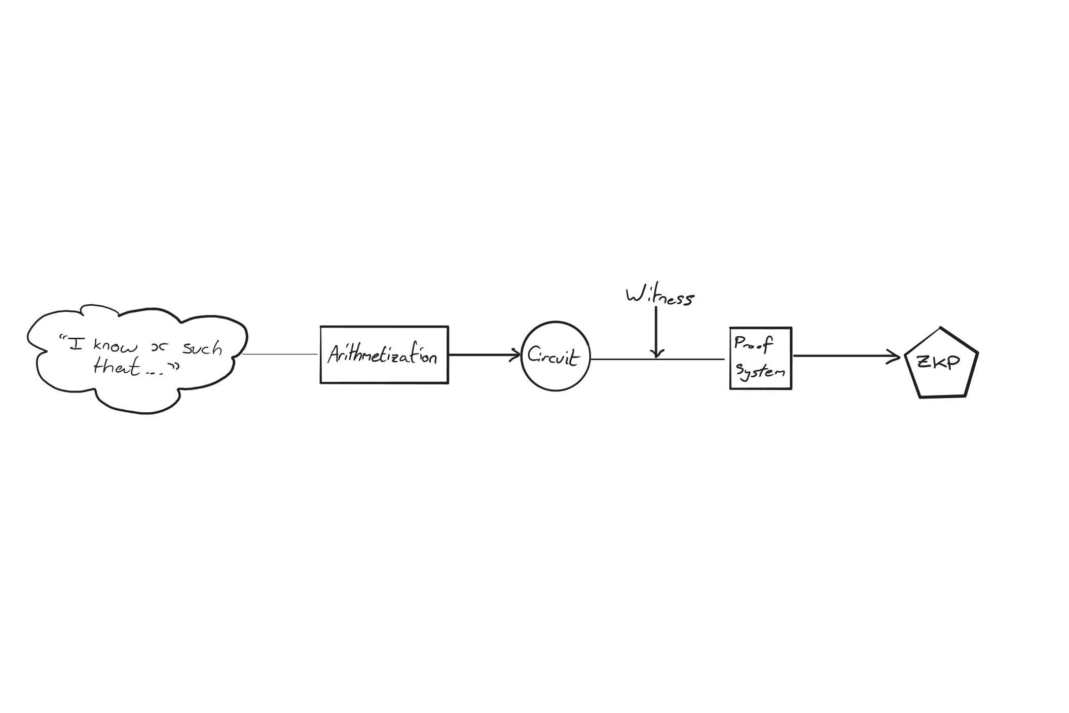
On a practical level, we can think of the step-by-step process of generating a ZKP as follows:
- 1. Decide on a computation to prove as well as a ZKP system (which also includes a choice of arithmetization).
- 2. Find a valid solution to the computation (the “witness”).
- 3. Use the arithmetization to generate a circuit that represents our computation.
- 4. Apply the proof system to the witness and circuit to generate a ZKP.
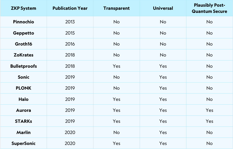
Below, we detail a time-ordered selection of some of the ZKP systems that have been developed so far [11] [12] [13] [14] [15] [16] [17] [18] [19] [20] [21] [22] [23].
3.6 SNARKs and STARKs
SNARKs are a type of argument of knowledge, commonly used with another process to make it a zkSNARK, a SNARK that is also a ZKP. We have previously covered the meaning of non-interactive – that a SNARK is succinct means that the proof size and verification time are relatively short (certainly shorter than the obvious proof of showing someone the answer to that which you are trying to prove).
They were first defined in a 2011 [24] paper by Bitansky, Canetti, Chiesa, and Tromer, who defined them in an effort to create a general proof system that was efficient enough to be used in practice. Their implementation involved expressing a computation as an R1CS, encoding it using elliptic curve cryptography, then giving validity conditions that the verifier could use to assure themselves of the proof’s validity. Many subsequent ZKP systems have been based on this work, operating with many of the same core mechanics.
The power of a general proof system is significant. For example, it can be used to prove that a series of valid transactions leads from one chain state to another without describing the transactions, vastly reducing the communication complexity without compromising on trustlessness. Prior to this development, this would have been possible but completely impractical – it would have involved composing a new kind of zero-knowledge proof for every computation you wanted to prove, such as the one we explored for proving knowledge of a discrete logarithm.
However, there were two pitfalls of many early implementations. Firstly, while the verifier had convenience in relatively short proof lengths and verification times, the prover would often take on a significant amount of work in computing the proof in the first place. Secondly, many required something called a ‘trusted setup’, a process to ensure the security of the cryptography used in the proof system. It involves generating cryptographic content that must be unknown to any individual, otherwise proofs can be falsified. While it can be conducted by a group of individuals such that a high level of security is present, it can actually be eliminated altogether.
Ben-Sasson, Bentov, Horesh, and Riabzev wrote a paper [25] in 2018 in an attempt to address these issues, defining Scalable Transparent Arguments of Knowledge (“STARK”). Scalability refers to a certain efficiency of the prover, and transparency refers to the absence of a trusted setup. They constructed an example of such a scheme based on Reed-Solomon codes, a method of encoding polynomials used in many modern applications, and they used AIR as the arithmetisation. This would go on to be the proof system used by StarkWare (founded by Ben-Sasson, Chiesa, Kolodny, and Riabzev) for their various products. Notably, their scheme can also be realised as non-interactive (explicitly mentioned in the paper), making it a type of SNARK if we do so, though different from many of the original SNARK implementations due to the lack of a trusted setup and a very different method of introducing zero-knowledge.
Notably, the categorisations of SNARK and STARK can have overlap. For example, a non-interactive STARK with an efficient verifier/proof size fits the definition of a SNARK.
Furthermore, a particularly important note is that STARKs and SNARKs are not necessarily zero-knowledge proofs by default – they are just arguments of knowledge. Many implementations are turned into zkSNARKs and zkSTARKs by introducing some kind of cryptographic layer that hides the extra information, but we should be careful to specify this where appropriate.
3.6.1 Trusted Setups
Many types of early SNARK implementations (specifically, many of those that are based on elliptic curve cryptography) require something called a ‘trusted setup’. In generating these proofs, there is a part of the setup that nobody must have access to, else they can falsify proofs. This is much the same as in the discrete logarithm example we explored earlier, where a prover who knows which requests will be made, can fool the verifier.
This secret part of the setup is a series of exponents used to generate elliptic curve points used in proof generation. Participants might trust a third party to generate these points and subsequently discard them, but in a web3 context, Trustlessness is a non-negotiable.
The alternative method is to perform this with a group of people who each add some randomness to the setup. As an overview, the process works similarly to the following: First, we specify a generator point for an elliptic curve, say, . Then, we repeat:
- 1. Participant n generates a random integer less than the order of the curve.
- 2. They calculate , obtaining the second factor from the previous person (note that person 1 just uses ).
- 3. They publish the result of their calculation and discard .
Now we know that if just one person has discarded their integer, then the exponent of the final point cannot be obtained.
The diagram below illustrates how the security of the setup works. If even one link in the chain (the secret share of one of the participants) is broken (deleted), then the attacker cannot reasonably succeed.
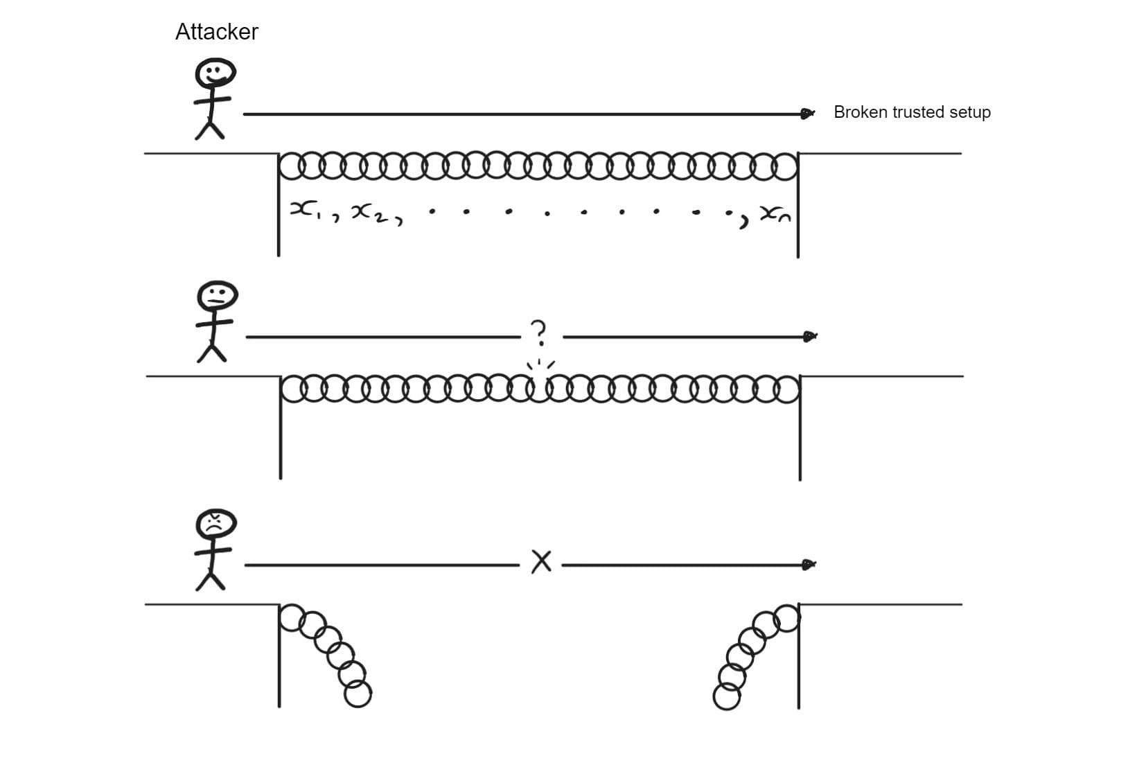
Of course, this does not eliminate trust completely – perhaps (however unlikely it is) all the participants colluded and can now falsify proofs. However, it is a vast improvement over the original state, which involved putting complete trust in a single party.
An example of this in practice can be found in the proto-danksharding ceremony conducted by Ethereum (currently in progress, as of writing). They are using polynomial commitments like those used in SNARKs to decrease data storage costs on Ethereum. The trusted setup involves a large number (>110,000) of participants, those being anybody who wishes to participate. This particular setup was designed particularly creatively – the randomness involved is captured from mouse movement and a password determined by the participant (as well as some system randomness). The software involved is open-source and run in-browser. By sourcing so many participants, and allowing anyone to join in, there can be a high degree of certainty that at least one person was trustworthy. More than this, if you only trust yourself, you can participate directly to be certain that the commitments are secure.
3.6.2 Elliptic Curves
Elliptic curves are curves of the form . These initially seem somewhat mundane, but we can actually define arithmetic on these points that becomes very helpful in designing cryptographic techniques.
Note that throughout this section we work with modular arithmetic – i.e. we perform all of our calculations as the remainder after division by some large number.
As we see in the below diagram, we define addition by saying that the point ‘at infinity’ is zero, and that any three co-linear points add to zero (counting the zero point if there is no third, and double-counting tangents). Then, we can define multiplication by whole numbers by saying that, for example, .
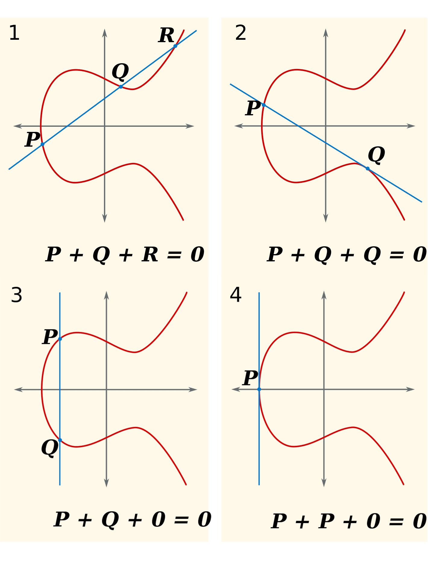
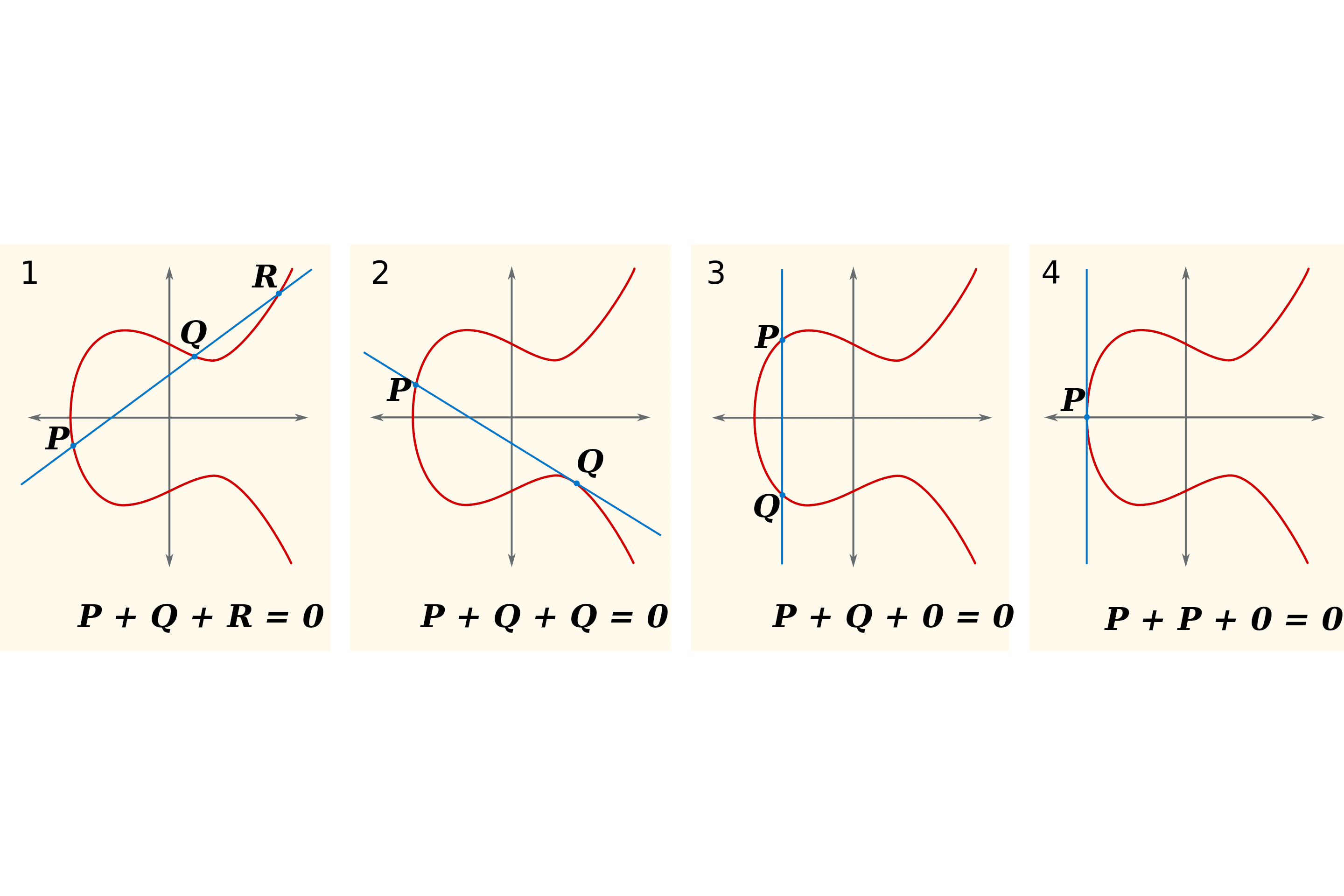
When we define arithmetic in this way, it becomes very hard to somehow ‘divide’ two points. By this, I mean that if I calculate and give you and , then you will find it very hard to find . This becomes incredibly useful for zero-knowledge, because we can perform arithmetic on these points and reason about the results without giving up the multiplier (perhaps something we want to keep secret).
Another important concept is that of bilinear maps. These are functions that take two elliptic curve points and give back some number, and moreover we can take multipliers out as exponents – i.e. we can do things like . Now we can compare these multipliers without revealing them (recalling the discrete log problem). This is useful because we can prove that someone must have used the same secret without us having to know what the secret is – as we might want to do when authenticating someone by password when they don’t want to give it to us directly.
The actual applications of these facts become more apparent when delving into the details of how ECC-based ZKPs (such as early SNARKs) work. Put concisely, they work by hiding our secret in the multipliers mentioned above, then letting the verifier confirm that they satisfy certain validity conditions by using bilinear maps.
3.6.3 Reed-Solomon Codes
Reed-Solomon (“RS”) codes are a commonly used way of encoding polynomials such that certain errors can be detected and even fixed. Put briefly, this is done by evaluating the polynomial at a number of points in excess of the degree of the polynomial, meaning that even the loss of a few of these points leaves us with enough information to reconstruct it.
Classically, this has been used for the storage and transmission of data – for example, in CDs and barcodes so that even if the medium is damaged, the data can still be read. Another interesting one is its use in sending pictures taken by the Voyager probes, useful here since the transmission of information through space introduces a lot of interference.
However, for our purposes, we are more interested in how this can be used to generate a ZKP.
Where the original SNARK used elliptic curves, ZKPs based on the original STARK use RS codes. By writing the statement of our proof into a low-degree polynomial, we can construct a proof of knowledge where we just have to show that we know a member of a certain RS code. By using suitably complex RS codes, we can make it unreasonably difficult to come up with a valid codeword without knowing the secret.
3.7 Proof Recursion and Incrementally Verifiable Computation
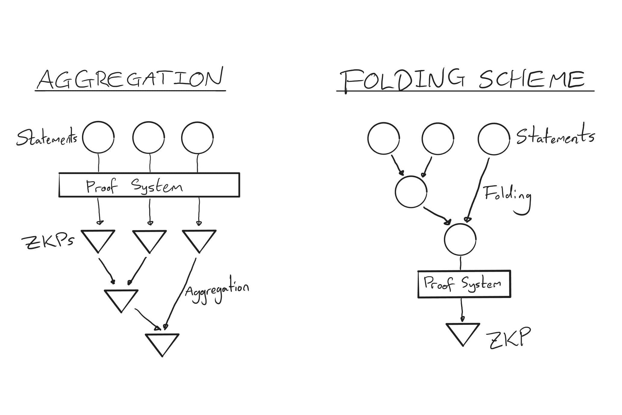
Proof recursion is the combination of a number of ZKPs into just one, which is then a proof of all the original statements.
A seemingly reasonable suggestion here is to just generate a ZKP for all the statements at once in the first place. However, recursion comes with a number of benefits.
Firstly, this is a convenient manner by which we can start parallelizing ZKP computations. Particularly in decentralized computing, we can delegate the task of generating each component ZKP to a number of machines, and hopefully apply a relatively efficient algorithm to compile all of these proofs.
If we want to prove the validity of a block, for example, this becomes even more interesting – speaking on a slightly oversimplified level, we can generate proofs of validity for the execution of each transaction on multiple different machines, then compile these into a proof of the whole block, which will be cheaper to verify than verifying each of the component proofs.
Secondly, certain ZKP systems benefit from better efficiency when applying these schemes. Up to a point, breaking down the computation can result in fewer resources used than simply producing a single proof.
Incrementally verifiable computation (“IVC”) is a type of proof recursion in which someone executing a program can, at each stage, prove that they are doing so correctly. It is a form of recursion since we are producing ZKPs that are accumulating each prior step’s proof. This has very interesting implications in Web3 – it means that we can perform a series of calculations in a trustless manner without the need for a consensus mechanism based on a large group of validators. Note, however, that avoiding censorship is a little more complex – if a small group is running the network, and they choose to censor certain transactions, then the ZKPs involved do not necessarily prevent this. It must be intentionally designed against.
The reason this is so helpful for our use case is that this model caters perfectly to how a blockchain operates. We continually apply a state transition function to the chain’s state with every transaction/block, and if we can generate a proof of validity at each step, we can make consensus very efficient. This is the foundation for zero-knowledge rollups, which we explore in more depth later in this document.
An obvious method of performing IVC (and the one introduced by its defining paper [26] in 2008) is to produce at step n a proof of the step and a proof of validity of the proof from step n-1. This is a bit of a mouthful, but we are just creating a proof by induction that we have executed the program correctly. This works perfectly well, but we can get much more efficient than this – for example, by using a folding scheme, the technique we cover in the next section.
3.8 Folding Schemes
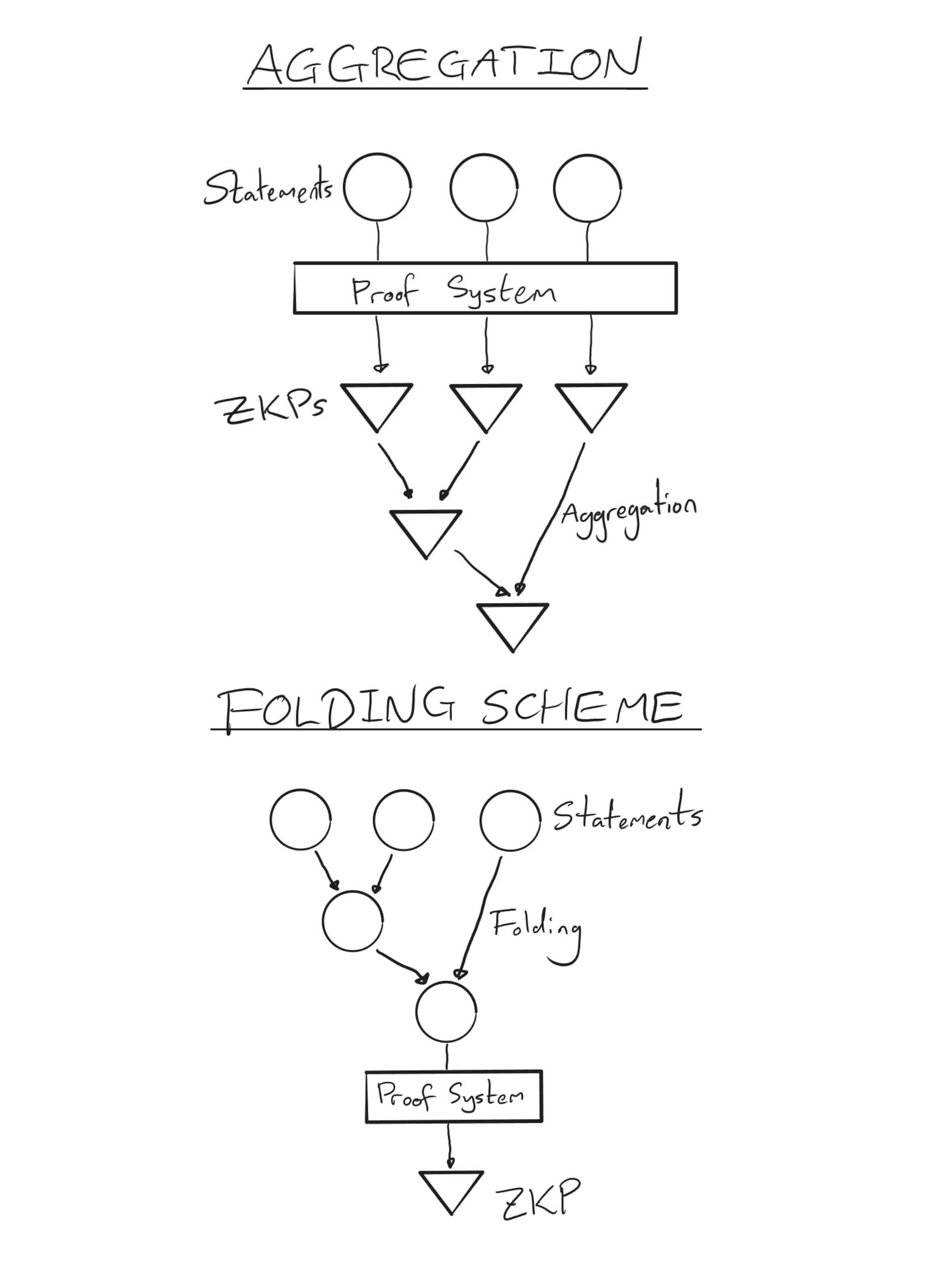
Another IVC method is ‘folding’. Instead of generating a ZKP at each step, we ‘fold’ the condition of validity for each step into a single condition that is satisfied only if each step of the computation was performed correctly. We then generate a ZKP of the truth of this condition. This has large computational savings over the previously mentioned method.
The below diagram illustrates the difference between recursively generating proofs and using a folding scheme. Once we move past the vertical line, we generate a ZKP at every move. With classic recursion, this becomes very expensive, because so many proofs must be generated. A folding scheme, on the other hand, requires much less computation, only generating a ZKP for the folded condition at the end of the process.
3.8.1 Nova, SuperNova, & Sangria
Folding schemes were first defined in the Nova paper [27] in 2021, Nova being the implementation defined in said paper. It could operate on computations of the form , where we can think of as a sort of state transition function, and where computations were expressed in the form of R1CSs. In other words, we’re thinking about the computation as being one machine that gets applied to our data at every step. A notable feature was that it introduced very little overhead (constant, dominated by two operations of order the size of the computation) and required only a single SNARK at the end.
While an exciting development, the difficulty with this model is that there is little flexibility. A single circuit has to be used that encompasses all possible operations. In other words, if we were implementing this for the EVM, you would need a circuit that covers every opcode at once, and use that circuit every time, no matter which opcode you wanted to use.
SuperNova [28] (2022) improves this process by allowing each step of computation to be defined by a different function with its own circuit, allowing for more adaptive systems (operations can much more easily be added) and giving rise to performance benefits (a universal circuit is not necessary, saving on space and processing). In the previous example of the EVM, we can write a circuit for each opcode and apply them only when necessary.
The remaining limitation was that both of these operate with R1CS constraints. Plonkish constraints are becoming more popular in part due to their suitability for use in proving computations, and neither Nova nor SuperNova were designed to handle them.
Sangria [29] (Feb 2023) went in a slightly different direction, adapting the work from Nova for the PLONK arithmetization. Unfortunately, this improvement came with a compromise in efficiency, introducing a greater overhead.
3.8.2 HyperNova
HyperNova [30] (Apr 2023, a recent advancement on SuperNova) generalised the work from the previous three. It defines a generalisation of the Plonkish and R1CS arithmetizations, and keeps SuperNova’s feature of allowing for a number of different circuits. More than this, it avoids the overhead that Sangria introduced, giving rise to a very general, adaptable, and efficient folding scheme. It remains to be seen the impact that this will have on related technologies, but we anticipate that it will enable significant developments.
The paper also introduces a new feature – ‘nlookup', which is an argument that is used to check the inclusion of certain values in the execution trace. Lookup arguments are particularly useful as they allow for optimisation techniques not otherwise possible, especially in the case of folding schemes. As per the HyperNova paper, nlookup “provides a powerful tool for encoding (large) finite state machines” (such as those used in blockchains, a key application). The optimisations come from the fact that lookup arguments enable us to break a computation down into pieces, and have the main computation “look up” the values from the components for its execution, instead of trying to contain all of the information in the table at once. For example, when proving a transaction, we might want to record the execution of a standard yet complex function (like a signature) separately, then feed this back into our circuit for the overall transaction.
History of ZKPs
ZKPs were created by Shafi Goldwasser, Silvio Micali (notably the founder of Algorand), and Charles Rackoff in their 1985 paper “The Knowledge Complexity of Interactive Proof Systems” [31]. The initial step was their description of interactive proof systems, in which two parties undertake a computation together, with one trying to convince the other of a certain statement. They also introduced the concept of ‘knowledge complexity’, a measure of the amount of knowledge transferred from the prover to the verifier. The paper also contained the first ZKP for a concrete problem, which was the decision of quadratic nonresidues mod m. The three authors (along with two others whose work they made use of) won the first Gödel prize in 1993 [32].
The next major development was that of non-interactive ZKPs. These are ZKPs where the verifier can verify the supplied proof without interaction from the prover. Blum, Feldman, and Micali showed in May 1990 that a common random string shared between the two is sufficient to develop such a protocol [33]. Non-interactive ZKPs were a significant development in the space, as it meant that proofs became verifiable without restriction on the communicating capacity of the prover/verifier. Furthermore, proofs could be verified in perpetuity, regardless of the continued engagement of the prover.
Impagliazzo and Yung would go on to show in 1987 that anything provable in an interactive proof system can also be proved with zero-knowledge [34]. Goldreich, Micali, and Widgerson then went one step further, showing in a 1991-published paper that (under the assumption of unbreakable encryption) any NP problem has a zero-knowledge proof [35].
In March 2008, Paul Valiant released the defining paper for IVC. The key contribution of the paper was to explore the limits of the time and space efficiency of non-interactive ARKs, defining a scheme that illustrated the results and could be composed repeatedly. The motivation for all of this was stated to be the implementation of IVC.
January 2012 saw a paper by Chiesa et al [36]. which coined the term “zk-SNARK” and introduced the practical creation of non-interactive ZKPs that could be used to demonstrate knowledge about algebraic computations.
In April 2016, Jens Groth released a paper detailing a SNARK that would become particularly popular.
Bulletproofs were first outlined in December 2017 in a paper from the Stanford Applied Cryptography Group [37], which introduced them as a non-interactive ZKP intended to facilitate confidential transactions.
In March of 2018, StarkWare published a paper in which they outlined their new idea, zk-STARKS, addressing security issues such as a lack of post-quantum security, as well as issues to do with applying ZKPs at scale. The paper itself states its motivation that early designs of efficient ZKPs were “impractical”, and that no ZK system that had actually been implemented had achieved both transparency and exponential speedups in verification for general computations [38]. Since then, there have been a number of (particularly technical) developments, such as advancing the efficiency of verification in the case of the FRI protocol [39] (released 12th Jan 2018).
In August of 2019, Gabizon, Williamson (co-founder of Aztec), and Ciobotaru submitted a paper describing PLONK – a SNARK with a universal setup, meaning that a trusted setup was no longer necessary for most uses. A trusted setup is a procedure used to generate a common piece of data that is used in every execution of a cryptographic protocol. While previously this had to be performed for every implementation of SNARKs, this development allowed people to use a single universal setup, which required the honesty of only a single participant to be secure, and could be contributed to in the future by new participants [40].
Folding schemes were first described in March 2021 by Kothapalli, Setty, and Tzialla, in their paper on Nova [41]. In December of the following year, Kothapalli and Setti would go on to improve this work, releasing SuperNova [42], which removed the need for universal circuits. In February 2023, Nicolas Mohnblatt of Geometry released the paper on Sangria [43], which allowed the work from Nova to be applied to a variant of the PLONK arithmetisation. However, Kothapalli and Setti then released in April their paper on HyperNova [44], generalising some of their previous work to CCS.
Applications of ZKPs
Within the Web3 space, there are two key applications of ZKPs.
1. Verifiable Computation: As blockchains have developed, many experience issues with scaling and transaction fees. Rollups are ‘extensions’ to a chain that bundle transactions and prove their validity on the original chain. One method of doing this is by generating a ZKP of the bundle and having it be verified on the base chain. In this case, we refer to it as a zero-knowledge rollup (ZKR).
Another method is to do this on a computation-by-computation basis, with users making requests to an execution network and the network responding with the output and a reference to the proof (or perhaps a validation of the proof). We refer to this construct as a ‘proving network’.
The popularity of ZKRs has grown significantly in recent times, with some of the largest players being zkSync, Polygon, and StarkNet. Each of these have their own approach to implementing ZKRs, with StarkNet standing out as being developed by the creators of STARKs (the other two using SNARKs).
Proving networks are more up-and-coming. Players of note here include RISC Zero and Lurk Lab. The main component is the zkVM, which executes and proves computations. Again, there is no agreement on what form of ZKP is better, with the former incorporating STARKs and the latter SNARKs. Folding schemes play a particularly important role in Lurk’s implementation - they make proof generation much more efficient and allow for more flexibility, such as proving execution in different VMs.
Something akin to a universal ZKR can be created here, by designing a L2 centered around receiving requests from smart contracts and returning the result with a proof of computation (or perhaps a reference to the validation of such a proof). Alternatively, the VM used to generate such proofs could be used in a ZKR directly. These ought to be mentioned in a more specific capacity, partly to show the close parallel with existing ZKRs but also to demonstrate that their products have broader use cases than just L2s.
The key difference here is that ZKRs operate in a manner much closer to an L1. From the user’s perspective, ZKRs operate as a blockchain, but this alternative operates more like a trustless version of a classical computer. It could be argued that the latter is a generalisation of a ZKR.
With these, there is a little more room for deciding which cryptographic solution fits better. Costs must be kept low, but if proofs are being served not to a chain but directly to a user, then the prover and verifier become much more balanced in how they are weighted. This comes from the fact that if the verifier is executed on-chain, then the consensus mechanism typically involves a number of nodes running the computation themselves and communicating their results, whereas if a single user wants to execute it, it only needs to be run the once, in isolation. The former is preferable when the proof needs to be verified by an on-chain component or by parties unwilling to verify themselves, where the latter may be preferable if only the user themselves need be convinced by the proof.
For recursion schemes, the sheer efficiency of folding schemes makes many other options nonviable, at which point it comes down to which one we use. With the recent release of HyperNova, much of the existing work done on folding schemes can be taken advantage of at the same time. Conversely, since the paper is quite recent, there is a case to be made for using an older, more reviewed method to provide higher security guarantees.
Outside of crypto, we encounter a number of other applications for verifiable computation.
- 1. Medical records: Selectively revealing relevant medical information as-and-when necessary.
- 2. Identity/membership: Proving an aspect of your identity, such as falling in a certain age range, or belonging to a certain group, without disclosing your exact identity.
- 3. AI: Owners of a proprietary model can run it without disclosing the model itself or its workings, and users can be sure that the claimed model is actually being run.
- 4. Scientific computing: Certain areas of research like genetics can require large amounts of computing, distributed or otherwise. ZKPs would help to ensure that aggregated computations are correct, or serve to quickly verify research that would take many hours to replicate.
- 5. Critical infrastructure: Ensuring zero fault tolerance in distributed infrastructure whose errors could risk lives, such as military defence networks.
- 6. Overall, the off-chain applications mostly fall into cases where a program is of a critical nature, or when there is some sort of adversarial nature to an interaction between parties, especially one where information needs to be concealed.
Overall, the off-chain applications mostly fall into cases where a program is of a critical nature, or when there is some sort of adversarial nature to an interaction between parties, especially one where information needs to be concealed.
2. Privacy: Another issue with many of today’s chains is their lack of privacy. Neither companies nor individuals particularly want their financial activities to be fully visible, nor do they want to disclose any sensitive information on a public chain. By using ZKPs to prove the validity of a transaction (or correct state change), the information contained within that transaction can be kept secret.
The issue of privacy in blockchains is a long-standing one. Monero, ZCash, and Aztec are all privacy-enabled chains [45], with Monero notably going in a different direction and using another type of ZKP called a Bulletproof.
Moreover, this applies at the application level as well. We might consider the use case of decentralised identity. Individuals may wish to prove that they belong to a certain group of people without revealing further details about their identity, perhaps to authenticate their use of an application. Here, ZKPs could be used to prove these details whilst keeping further information private.
For many of these, the way in which cryptographic techniques are implemented can vary significantly. Any decision over which to use will depend heavily on the details - for example, Monero use Bulletproofs rather than SNARKs, indicating that there are cases where even a less general proof system may be preferable. However, it might be expected that when comparing between suitable candidates, many of the topics mentioned previously would factor in.
Appendix
6.1 Arithmetisations
6.1.1 R1CS
This explanation comes with great help from Vitalik’s guide [46], from which further information can be found.
First, we decide on the computation we want to prove. For the purposes of demonstration, let's go with “I know such that ”. The answer for real is 3 (there are two other complex solutions), but of course for the purposes of this discussion we don't want to reveal that.
We then ‘flatten’ the equation, converting it into a series of simpler statements of the form , where can be addition, subtraction, multiplication, or division. These statements are called gates. In this case, we work our way down to
Expanding these, we see that , which was the calculation we wanted to make in the first place. We break the computation into gates so that it is in the right form for the next step.
We re-write each gate as an R1CS. Note that we use the phrase to refer to the whole process, but this is because the R1CS is the defining feature. An R1CS is a collection of sequences of three vectors with another vector s (the solution/commitment to the R1CS) such that
Each R1CS represents a gate, and each row a variable - including a constant 1. In this example, we let s contain in order and . For each gate, we obtain
We can see that putting these (as well as ) into the equation gives us back each gate in order. The witness is .
Now we convert the R1CS into a Quadratic Arithmetic Program (QAP), which is again the same logic but in polynomial form. Before digging into this, we'll quickly describe Lagrange interpolation. This is a method of finding a polynomial that passes through a given set of points. For example, suppose that we want a polynomial passing through , and . It isn't obvious which polynomial should work. If the values at these points were zero, we could just take - so first, we make the problem slightly easier, and we consider a polynomial passing through , and . We're going to do this for each point, and then add all the polynomials together, giving us the result we want.
When we consider this first step, it turns out that it is actually quite easy to achieve. First, we look at . This has values of zero where we want them, and it sticks out somewhat at , with a value of 2 at that point. So we re-scale, and take , which gives us the values we want. Repeating this for the other two points, we get and . Then we add them together, to obtain , which we can verify passes through all of our points.
A general formula for a polynomial passing through all points for a finite range of is this:
We now use Lagrange interpolation to generate a series of polynomials for the collections of and in turn, so that in the case of a, evaluating the -th polynomial at gives the n-th value of the -th a vector.
The point of this is that by doing this we can express the R1CS constraints as one condition on the polynomials. Let , where is the -th polynomial as mentioned above. Repeat for and . Letting be some factor and be a polynomial, we consider the following equation:
We can see that checking the conditions is a simple matter of confirming that the left-hand side evaluates to 0 for each .
Note that since we know some of the roots of the LHS, we can let , and is the factor that the two differ by. In fact, instead of checking the LHS for equality to zero at each point, we perform polynomial division by and check that there is no remainder, thus verifying the same condition.
And this describes the arithmetisation. The combination of and attest to the statement that we know the solution to the problem we are creating a ZKP for. In practice, we communicate the polynomials as vectors containing their coefficients. Also, more often than not, we work over finite fields to avoid issues of accuracy (to see this, note that is as a float, which terminates in a computer's storage, but 4 in , losing no accuracy) and so that everything works better with elliptic curve cryptography, which becomes important when we start introducing the feature of zero-knowledge. All of the above steps still hold when we do this, but we perform all calculations using modular arithmetic.
6.1.2 Plonkish
This description was much informed by Aztec’s guide on the subject [47]. To describe PLONK-like arithmetisations, we go through a few levels of generality.
6.1.2.1. AIR
The idea will be to express any repeated computation as a set of polynomial constraints, then demonstrate that we know what the computation outputs after however many steps.
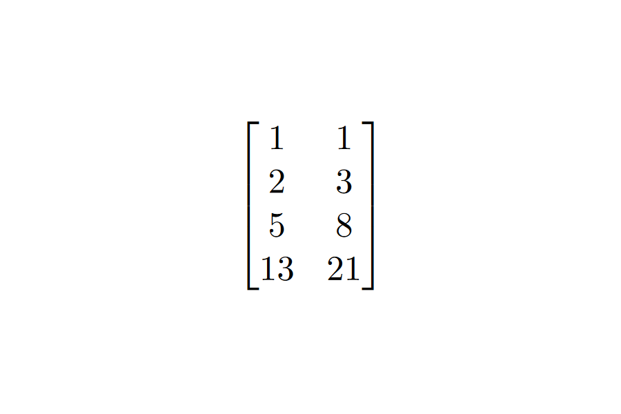
We begin by expressing the `state' of the computation at each stage as a row of variables. The idea will be that we can give any two consecutive rows to the constraints and fulfill them. Let's use the Fibonacci sequence as an example. We only need two numbers to continue the sequence, so each row will contain two consecutive Fibonacci numbers. We then decide on the conditions under which these rows are valid. In this case, if we let be one row, and the next, then the conditions in question are and - i.e. we take the polynomials to be and . Building out the table, we get the following:
The AIR is the set of polynomials {}, and the execution trace is the table above. We decided initially that the polynomials would be of degree 1, and that each would operate over 4 variables. We say that the AIR has a width of 2 and a length of 4 (the dimensions of the table).
Formally, an AIR over a field is a set of constraint polynomials {} over of a certain pre-defined degree . An execution trace for is a collection of n vectors from - or perhaps an element of . is valid if for all and in and for all . We say that has length and width .
6.1.2.2 PAIR
In these, we add a number of columns to the trace: columns . These are commonly called ‘selectors’. We expand the constraint polynomials accordingly, now having inputs. The point of this is to allow for different constraints for specific rows.
For example, if we wanted to interrupt our last example on row 4 and insert a different operation, say, , then we could take , and we let be zero except for at position 4, where it is 1.
6.1.2.3 RAP
Finally, we consider the Randomised AIR with Pre-Processing (RAP). In this version, we allow the verifier to supply random field elements and the prover to add columns accordingly. This introduces verifier randomness into the system, which is a key component of many ZKP systems. A good example of this is the one we illustrate at the beginning of this report, where the prover wants to show that they know a discrete logarithm, and in each round the verifier requests one of two variables, randomly, for the prover to hand over. RAPs are the most general form of the arithmetisation used in PLONK.
6.2 Sharks and Starks
6.2.1 Snarks
Vitalik’s guide on ECC-based SNARKs is excellent [48], and formed the foundation for this description.
The underlying security assumption of SNARKs is the knowledge-of-exponent assumption (KEA):
For any adversary A that takes inputs and returns with , there exists an extractor which, given the same inputs as , returns such that .
The process of forming a SNARK is as follows:
- 1. First, form an R1CS circuit of the problem (as described previously).
- 2. We next perform the trusted setup. As part of the protocol, we specify a random elliptic curve point $G$, called the generator. Take values and , and calculate the pairs for all and across and then for all . Those first five values MUST be discarded. Due to the DLP, they cannot be retrieved from the curve points, and due to KEA, we then know that any points of the form (note that we can check this with a bilinear pairing and the trusted setup) must represent a linear combination of the polynomials we generated. We also include up to a suitable power, for use in the last step.
- 3. To prove the statement, the prover must calculate and , along with the same for and . The prover doesn't (and shouldn't) know to compute these - rather, they can be calculated as linear combinations of values in the trusted setup.
- 4. The prover also needs to show that the s used in each of and is the same. They generate a linear combination with the same coefficients using the last values added to the trusted setup, and we use the bilinear pairing again to check that this is valid.
- 5. Finally, we need to prove . We do this with a pairing check of , where , which we can generate using the values of .
6.2.2 Starks
This overview was informed by the original STARK paper [49].
The process of forming a STARK is described below. We reference a number of processes that we will go on to describe in more detail.
- 1. Express the computation as an AIR, described previously.
- 2. Transform the AIR into an `algebraic placement and routing' (APR) reduction. This involves expressing the AIR as an affine graph, with states as nodes and edges as state transitions.
- 3. Use the APR representation to generate two instances of the Reed-Solomon proximity testing (RPT) problem via a 1-round IOP. This step is referred to as the algebraic linking IOP (ALI) protocol.
- 4. For the witnesses generated in the previous step, the fast RS IOP of proximity (FRI) is applied.
The APR is designed to optimise the arithmetisation of the computation we are trying to prove. The idea of this step is to express the circuit as a certain subset of the 1-dimensional affine group over a finite field, specifically an affine graph. In some sense, the algebraic nature of the affine group is such that when we do this, we get a more efficient encoding of the statement we are trying to prove.
The RPT problem is, in essence, a problem of showing that two polynomials are suitably similar. ALI is the process by which we turn our statement about a computation into one about polynomials, and then express this as a ZKP by running it as an interactive oracle proof (IOP). We have already seen, in the case of SNARKs, that using polynomials gives a `nice' form for our statements that is easier to write ZKPs for.
Finally, FRI. This speeds up the proof generated in the previous step, and makes it more practical for use. It has a few effects.
The proof from ALI is interactive. A back-and-forth process is limiting, so FRI reduces it such that the prover sends the verifier the proof, and no more interaction is needed.
The prover and verifier complexities are reduced.
The work done by the prover can be completed in parallel, reducing the proving time to .
Footnotes
- 1.
A popular explanation for ZKPs used in many sources. While we are unsure of its origin, the earliest mention we found was in a 2008 lecture by Mike Rosulek at the University of Montana. https://web.engr.oregonstate.edu/~rosulekm/pubs/zk-waldo-talk.pdf
The source for the figures is a presentation by Beanstalk Network: https://docs.google.com/presentation/d/1gfB6WZMvM9mmDKofFibIgsyYShdf0RV_Y8TLz3k1Ls0/edit#slide=id.p
- 2.
This is called the “Ali Baba cave” example. Source: https://en.wikipedia.org/wiki/Zero-knowledge_proof
- 3.
This can refer to both the algorithmic complexity and the in-practice running time. We typically talk about the former in academic literature and high-level discussions of performance, and the latter when discussing individual implementations and their intricacies.
- 4.
- 5.
- 6.
- 7.
- 8.
- 9.
- 10.
- 11.
- 12.
- 13.
- 14.
- 15.
- 16.
- 17.
- 18.
- 19.
- 20.
- 21.
- 22.
- 23.
- 24.
- 25.
- 26.
- 27.
- 28.
- 29.
- 30.
- 31.
- 32.
- 33.
- 34.
Russell Impagliazzo, Moti Yung: Direct Minimum-Knowledge Computations. CRYPTO 1987: 40-51
- 35.
- 36.
- 37.
- 38.
- 39.
- 40.
- 41.
- 42.
- 43.
- 44.
- 45.
Note that Aztec is more accurately referred to as a ZKR.
- 46.
- 47.
- 48.
- 49.